Policy Optimization for RL and LLM Alignment — Theory

Modern large language models are typically trained in three steps:

1. First, you pre-train LLMs on a humongous amount of web-scrawled data.
2. Then, you supervised fine-tune (SFT) the pre-trained models on a large dataset consisting of “expert” prompt-response pairs.
3. Lastly, you post-train the models to “align” their behaviors with human preferences. Reinforcement Learing with Human Feedback (RLHF) is one popular approach.

During pre-training, models are effectively turned into general-purpose statistical machines that can decently predict the next token that follows a sequence of tokens. After this initial stage, models are better equipped with the knowledge of how to generate tokens given trillions and gazillions of tokens they have learned from, but they are not quite useful yet for real tasks, so we subsequently instruct them in a supervised way how to generate better responses by exposing them to labeled input-output pairs. However, this is a rather expensive procedure due to the challenges of collecting such datasets, and SFT alone may not be sufficient. The models might have learned how to craft accurate information, yet the model behaviors could certainly diverge from our expectations of how models should respond. The supervised fine-tuned models could generate subpar responses for creative tasks, since the SFT phase had still been all about maximizing the likelihood using autoregressive next word prediction. Even worse, models might generate responses that are biased, harmful, overly formal, or lengthy, just to list some of the undesirable traits for an LLM response. RLHF is a technique that addresses these shortcomings to better align models’ responses with our expectations. The way we do it is by training a reward model by telling them about our preferences, and using it as a proxy to update the LLMs’ behaviors, or “policy,” to borrow RL terminology.

RLHF is not a form of sorcery specifically invented for LLM post-training, but it is undoubted that it has immensely contributed to a revolution that has rendered LLMs more helpful and safer. The pioneer of this revolution, which has traditionally been an integral part of the alignment research, as it pertains to LLM alignment was OpenAI’s InstructGPT, which was trained using RLHF on top of GPT-3. It is shown to generate responses preferred by human lebelers and show improvements in truthfulness of the responses, while still excelling at traditional NLP tasks as tested on conventional benchmarks¹1 Ouyang et al. (2022), Training language models to follow instructions with human feedback . Anthropic also showed that RLHF improves LLMs’ performance, but also notably accentuated that the mechanisms of RLHF based on preference modeling could function as a double-edged sword, raising concerns for censorship, fraud, and misinformation²2 Bai et al. (2022), Training a helpful and harmless assistant with reinforcement learning from human feedback .

The north star of this post is to lay out the details of alignment in a granular way, with a particular focus on the optimization algorithms used to update the policy, among which we’ll discuss PPO, GRPO, and DPO.

Basic concepts in RL

Agent, state, action, reward, and trajectory

An RL agent interacts with the world it is situated in by receiving the (potentially incomplete and fragmentary) information about the world, which we refer to as states. It takes an action given its knowledge of the world, and receives a reward³3 It is possible for the reward to be deferred until the end, rather than after each action is taken. , where a high reward indicates to the agent that it was a promising action to take, hence increasing the likelihood of taking the same action in the future. Along with the reward, the agent receives a new state.

To articulate this a little more mathematically, we can first define the state space \(\mathcal S\) and the action space \(\mathcal A\) representing the set of all available states and actions the agent can take. At time step \(t\), the agent has access to state \(s_t\); takes action \(a_t\); and receives reward \(r_t\) and a new state \(s_{t+1}\). A trajectory, denoted as \(\tau\), is a sequence of states, actions, and rewards that has happened. Oftentimes, \(T\) is reserved as a symbol that denotes the terminal timestep, so a trajectory from timestep \(t\) to \(T\) can be expressed as \(\tau = (s_t, a_t, r_t, s_{t+1}, a_{t+1}, r_{t+1}, \cdots, s_T)\).

Policy, policy gradient and basic policy gradient algorithm

A policy of an RL agent, often denoted as \(\pi\), decides which action to take. A policy can be deterministic or stochastic: under a deterministic policy, a state is mapped to a specific action, while under a stochastic policy, the agent obtains the probability of taking a specific action given the state. Mathematically, an agent following a deterministic policy \(\pi\) gets \(\pi(s_t) = a_t\), while it gets \(\pi(a_t \mid s_t) = p\), where \(p \in [0, 1]\), under a stochastic policy. A policy is often parameterized, meaning that learning to optimize a policy involves updating the parameters of a model, which could be a deep learning model, for instance. In this post, we denote such parameters as \(\theta\).

It is also helpful to make a distinction between on-policy and off-policy RL. On-policy learning updates the policy using the data generated by the same policy. For off-policy learning, it is not necessary for the data to have been generated by the same policy. The pros and cons are clear: on-policy methods use fresh data from the current policy and are typically more stable (and less biased) with respect to the current policy distribution, while off-policy methods are usually more sample-efficient.

Consider a trajectory \(\tau = (s_1, a_1, r_1, \cdots, s_T)\), where \(T\) could potentially be \(\infty\) (to be a little handwavy), in which case we have an infinite trajectory. The training objective of RL is to maximize the expected cumulative reward over \(\tau\). There is some design choice concerning how we should define the cumulative reward: should we assign equal weight to \(r_t\) and \(r_i\) for \(i > t\), or should we prioritize \(r_t\)? We can represent both scenarios in a single equation by incorporating a discount factor \(\gamma \in (0, 1]\), which controls how much weight is given to future rewards. In the formula below, \(R(\tau)\) is the reward function representing the cumulative return over the trajectory \(\tau\): \begin{align} R(\tau) = \sum_{i=0}^{T - 1} \gamma^i r_i. \end{align} If \(\gamma = 1\), we have \(R(\tau) = r_1 + r_2 + \cdots + r_T\), with all \(r_i\)’s equally weighted. On the other hand, as \(\gamma \to 0\), we more heavily weigh the immediate rewards. (YOLO!) Instead of considering the entire trajectory, that is, \(0 \leq i \leq T - 1\), we can consider a smaller interval \(t \leq i \leq T\) and define reward-to-go as follows, which tends to be more stable:

$$ \begin{align*} G_t = \sum_{i=0}^{T-1} \gamma^{i-t} r_i. \end{align*} $$

Using \(G_t\) instead of \(R(\tau)\) offers the benefit of lower variance while still having the estimator unbiased. For now, we’ll stick to \(R(\tau)\). We’ll get a chance to revisit a relevant discussion in a section or two.

This naturally leads to the definition of the expected cumulative reward \(J(\pi_\theta) = \mathbb E_{\tau \sim \pi_\theta} [R(\tau)]\), the objective we try to maximize in training with RL⁴4 Here, I use \(R(\tau)\) but it is also commonly replaced with \(G_t\). In machine learning, \(J(\theta)\) is, as far as I’m aware, a common notation for the cost function of a model parameterized by \(\theta\). , with the optimal parameters being \(\theta^*\). To update \(\theta\), under this formulation, we can use the standard gradient ascent, \(\theta \leftarrow \theta + \alpha \nabla_\theta J(\pi_\theta)\). The subscript under \(\mathbb E\) also merits a closer look: our expectation is over the trajectories sampled from \(\pi_\theta\).

We are now ready to formally define the policy gradient, but in fact, we have already introduced it in the previous paragraph. The policy gradient is the gradient of the expected cumulative reward, \begin{align} \nabla_\theta J(\pi_\theta) = \nabla_\theta \mathbb E_{\tau \sim \pi_\theta} [ R(\tau) ], \end{align} and policy gradient algorithms are algorithms used to optimize our policy.

REINFORCE and baseline

Let’s derive the actual expression that we can implement to optimize \(\theta\). \((2)\) is mathematically simple, but its expectation is over \(\tau \sim \pi_\theta\). We can call the most basic version of our algorithm to optimize our policy, well, the vanilla policy gradient algorithm, but it actually has a better name: REINFORCE.

$$ \begin{alignat*}{2} \nabla_\theta \mathbb E_{\tau \sim \pi_\theta} [R(\tau)] &= \nabla_\theta \int_{\tau} p(\tau \mid \theta) R(\tau) d\tau \\ &= \int_\tau \nabla_\theta \, p(\tau \mid \theta) R(\tau) d\tau \\ &= \int_\tau p(\tau \mid \theta) \nabla_\theta \log p(\tau \mid \theta) R(\tau) d\tau & \quad (a) \\ &= \mathbb E_{\tau \sim \pi_\theta} \left[ \nabla_\theta \log p(\tau \mid \theta) R(\tau) \right] \\ &= \mathbb E_{\tau \sim \pi_\theta} \left[ \nabla_\theta \log \left( \mu(s_1) \prod_{i=1}^T \pi_\theta (a_i \mid s_i) \, p(s_{i+1} \mid s_i, a_i) \right) R(\tau) \right] \\ &= \mathbb E_{\tau \sim \pi_\theta} \left[ \sum_{i=1}^T \nabla_\theta \log \pi_\theta (a_i \mid s_i) R(\tau) \right] & (b) \\ &\approx \frac{1}{N} \sum_{j=1}^{N} \sum_{i=1}^T \nabla_\theta \log \pi_\theta (a_{ji} \mid s_{ji}) R(\tau_j), & (c) \end{alignat*} $$

where \(a_{ji}\) and \(s_{ji}\) denote \(a_i\) and \(s_i\) from \(\tau_j\). Here are some more details:

• \((a)\) Log-derivative trick is use here, which I’ve also written about in my VAE post.
• \((b)\) When \(\log\) expands to each term, \(\pi_\theta (\cdot)\) is the only term that depends on \(\theta\), making every other term cancellable.
• \((c)\) This is an unbiased estimator.

So far so good, but REINFORCE has some significant shortcomings:

1. In updating the parameters based on this gradient, we are using the reward of the entire trajectory, as evidenced by the \(R(\tau_j)\) at the end. Thus naturally, it has a large variance, which could render the training unstable.
   Takeaway: We need to modify the algorithm to reduce variance.

2. If the trajectory is too lengthy, this will lead to relatively few gradient updates, hence REINFORCE is sample-inefficient.
   Takeaway: We need a more sample-efficient approach.

How can we reduce variance? A good starting point is replacing the reward \(R(\tau)\) only computed at the end of the trajectory with reward-to-go \(G_t\):

$$ \begin{align*} \nabla_\theta J(\pi_\theta) = \mathbb E_{\tau \sim \pi_\theta} \left[ \sum_{i=1}^T \nabla_\theta \log \pi_\theta (a_i \mid s_i) \, G_i \right]. \end{align*} $$

Notice that the root cause of a high variance is the rewards fluctuating wildly. Replacing \(R(\tau)\) with \(G_t\) helps, but what if we can go one step further?⁵5 Baselines often do a great job as a variance reduction technique. Nevertheless, implementing the optimal baseline is not straightforwward. Moreover, as Chung et al. (2021) point out, introducing baselines may also affect learning dynamics in unexpected ways. Take a look at the following modified expression where we’ve replaced \(G_i\) with \(G_i - b(s_i)\):

$$ \begin{align*} \nabla_\theta J(\pi_\theta) = \mathbb E_{\tau \sim \pi_\theta} \left[ \sum_{i=1}^T \nabla_\theta \log \pi_\theta (a_i \mid s_i) \left( G_i - b(s_i) \right) \right]. \end{align*} $$

The term \(b(s_i)\) is called the baseline. Unlike REINFORCE, where the gradient was scaled by the absolute reward, this version changes the scaling factor to a number representing how much better or worse the outcome for a certain state was, relative to a baseline. Introducing \(b(s_i)\) can center the signal and thus reduce variance.

1. What is a reasonable baseline?
   A commonly used baseline is the on-policy value function, which gives the expected return given a (static) policy starting from a state:

   $$ \begin{align*} V^{\pi_\theta}(s_t) = \mathbb E_{\tau \sim \pi_\theta} \left[ G_t \mid s_t = s \right]. \end{align*} $$

   If starting from \(s_0\), \(V^{\pi_\theta} (s_0) = \mathbb E_{\tau \sim \pi_\theta} \left[ R(\tau) \right] \) by definition. Compare \(b(s_i)\) and \(V^{\pi_\theta} (s_t)\), and their similarity is apparent.

2. But where do we obtain the value function?
   Using \(V^{\pi_\theta}\) as the baseline only makes sense when we actually have the knowledge of the expected return starting from an arbitrary state, which is clearly not provided to us a priori. Well, if we don’t know what it is, then we can learn it! In practice, we train a separate neural network parameterized by \(\phi\) to estimate the value function. This model that learns to predict \(V^{\pi_\theta}\) is often called a critic. Recall that the baseline should be a good representation of the actual reward-to-go, which is obtained from actual samples. The critic’s training objective for \(V_\phi\) is thus to minimize the difference between \(G_t\) and \(V_\phi(s_t)\): the smaller the value of \(G_t - b(\cdot)\) is, the lower variance we can expect. If you hear “actor-critic” method, it is precisely referring to this family of algorithms where the actor (agent) learns to optimize its policy using the \(V\)-signals provided by the critic.

3. Wouldn’t it shrink the gradient?
   This is the beautiful part — the answer is no. Baselines don’t affect the expected value.

Some notational sidenotes and conceptual clarifications

So far, we’ve laid out all the necessary details for RL. When I was first learning about these concepts, I was fairly confused about the notations, some of which even appeared to be interchangeable at times. So I’d like to dedicate a short section to clarify on the notations.

Let’s start again with the policy gradient \(\nabla_\theta J(\theta)\). In the previous section, we introduced two versions, with the latter often enjoying a reduced variance:

$$ \begin{align*} \mathbb E_{\tau \sim \pi_\theta} \left[ \sum_{i=0}^{T-1} \nabla_\theta \log \pi_\theta (a_i \mid s_i) \, R(\tau) \right] \quad \text{and} \quad \mathbb E_{\tau \sim \pi_\theta} \left[ \sum_{i=0}^{T-1} \nabla_\theta \log \pi_\theta (a_i \mid s_i) \, G_t \right]. \end{align*} $$

So it turns out the only difference really lies in what comes after the gradient-of-log-prob expression. As also beautifully explained here, there, hither, and yon, we can define a generalized version of the policy gradient as:

$$ \begin{align*} \nabla_\theta J(\theta) = \mathbb E_{\tau \sim \pi_\theta} \left[ \sum_{i=0}^{T-1} \nabla_\theta \log \pi_\theta (a_i \mid s_i) \, \Psi_i \right] \end{align*} $$

where \(\Psi_t\) can be any of the following six forms:

• \(R(\tau)\): total reward of the trajectory
• \(G_t\): total reward of the trajectory starting from \(s_t\), introduced as “reward-to-go”
• \(G_t - b(s_t)\): reward-to-go with baseline
• \(Q^{\pi_\theta} (s_t, a_t)\): state-action value function
• \(A^{\pi_\theta} (s_t, a_t) \triangleq Q^{\pi_\theta} (s_t, a_t) - V^{\pi_\theta} (s_t)\): advantage function
• \(\delta_t \triangleq r_t + \gamma V^{\pi_\theta} (s_{t+1}) - V^{\pi_\theta} (s_t)\): temporal difference (TD) residual, where \(\gamma \in (0, 1]\) is the discount factor

More terms have been introduced but (I promise) we will construct a nice set of pairwise conceptual bridges very soon.

• \(Q\) is basically \(V\) after taking an action: The state-action value function is not a novel concept. While \(V^{\pi_\theta} (s_t)\) denotes the expected cumulative return starting at state \(s_t\) and following policy \(\pi_\theta\), \(Q^{\pi_\theta} (s_t, a_t)\) denotes the same quantity but crucially after taking action \(a_t\) at state \(s_t\), and then following policy \(\pi_\theta\). Formally, \(Q^{\pi_\theta} (s_t, a_t) = \mathbb E \left[ G_t \mid s = s_t, a = a_t \right] \).
• \(G_t\) and \(b(s_t)\) are Monte Carlo estimates: \(G_t\) and \(Q^{\pi_\theta} (s_t, a_t)\) look like twins, and so do \(b(s_t)\) and \(V^{\pi_\theta} (s_t)\). This is because \(G_t\) is a Monte Carlo estimate of \(Q^{\pi_\theta}(s_t, a_t)\) and \(b(s_t)\) also could be, when it is computed from sampled returns. (If it comes from a critic, it is a learned estimate of \(V^\pi\); more on this shortly.) This provides a justification to why we have \(G_t - b(s_t)\) as a possible form of \(\Psi_t\).
• \(A^{\pi_\theta}\) measures how good an action is: The advantage function is defined as \(Q^{\pi_\theta} (s_t, a_t) - V^{\pi_\theta} (s_t)\). Recall that we perform gradient ascent at step \(t\) to help our agent learn how to take the best action \(a_t\). The advantage function tells us how “advantageous” \(a_t\) is: if it is positive, it means that \(a_t\) was a promising action to take (since it is larger than the expected reward over all possible actions). The Monte Carlo estimate for \(A^{\pi_\theta}\) is \(\hat{A}_t = G_t - b(s_t)\).
• TD is a method that uses bootstrapping and updates more frequently: Previously, we replaced \(R(\tau)\) with \(G_t\) as a variance reduction technique. \(G_t\) still relies on the trajectory from time \(t\) until terminal. But what if the trajectory never ends (in other words, it’s continuous and not episodic)? The TD method is an effective solution here: it updates after each step, rather than waiting until the end. The change is simple: instead of using \(G_t\) or \(Q^{\pi_\theta}(s_t, a_t)\), we replace it with \(r_t + \gamma V^{\pi_\theta}(s_{t+1})\). As a result, this results in a form that is essentially the advantage, commonly using \(V_\phi\) estimated by the critic, which is often a neural network. It should be additionally noted that the TD residual is biased, and it is unknown if the TD method converges faster than the Monte Carlo methods. (Empirically, it does seem to converge faster, though.)⁶6 There is an interesting section on Wikipedia on the relationship between TD learning and neuroscience

---

TRPO

Fundamentals: Surrogate objective and trust region constraint

TRPO, which stands for Trust Region Policy Optimization, was first introduced in Schulman et al. (2015). The first sentence of its abstract decently summarizes its objective:

We describe an iterative procedure for optimizing policies, with guaranteed monotonic improvement.

The core idea of TRPO (and its descendant, PPO) is to constrain how much the policy can change per update to ensure monotonic improvement. Assuming the same parameterized policy \(\pi_\theta\), the update from \(\theta\) to \(\theta'\) involves maximizing the following surrogate objective:

$$ \begin{align*} \mathbb E_{\tau \sim \pi_\theta} \left[ \sum_{t=1}^T \frac{\pi_{\theta'}(a_t \mid s_t)}{\pi_\theta(a_t \mid s_t)} A^{\pi_{\theta}}(s_t, a_t) \right] \end{align*}. $$

The quantity \(\dfrac{\pi_{\theta'}(a_t \mid s_t)}{\pi_\theta(a_t \mid s_t)}\) is called the policy ratio, which assigns importance of varying degree to each action. Fixing \(s_t\) and \(a_t\) sampled from a trajectory⁷7 I think \((s_t, a_t) \sim \pi_\theta^{(i)}\) is a slightly unconventional notation that differs from how we’ve used it previously in this post, chosen to not clutter the notation. This expression should be understood as “picking out \((s_t, a_t)\) from a trajectory that follows the policy \(\pi_\theta^{(i)}\)”. , \(\pi (a_t \mid s_t)\) spits out the probability of choosing \(a_t\) at state \(s_t\), hence \(r_t(\theta) > 1\) signals \(a_t\) is more likely under \(\theta'\). For our objective is to maximize the surrogate objective, if the advantage is negative, the objective tries to steer away from the specific \(a_t\). Multiplying the policy ratio by the advantage \(A^{\pi_\theta} (s_t, a_t)\) achieves precisely that. By including the ratio of the new policy’s behavior relative to the old policy’s, we are explicitly taking into account the old policy as some kind of reference policy (to state informally). But TRPO adds a trust region constraint, constraining on how much the policy can change relative to the old policy using KL divergence:

$$ \begin{align*} \mathbb E_t \left[ D_{\text{KL}} \left(\pi_\theta (\, \cdot \mid s_t) \, \lVert \, \pi_{\theta'} (\, \cdot \mid s_t) \right) \right] \leq \delta \end{align*} $$

where \(\delta\) is the value denoting maximum KL divergence that we tolerate.

Monotonic improvement

An important part of TRPO is that it guarantees monotonic improvement. This proof builds on the identity from Kakade & Langford (2002): given two policies \(\pi\) and \(\pi'\) and the expected return of \(\pi\) defined as \(\eta(\pi) = \mathbb E_\tau \left[ \sum_{t} \gamma^t r_t \right]\),

$$ \begin{align*} \eta(\tilde{\pi}) = \eta(\pi) + \mathbb E_{s_0', a_0', \cdots \sim \tilde{\pi}} \left[ \sum_t \gamma^t A^{\pi}(s_t', a_t') \right]. \end{align*} $$

The identity tells us that if we have a positive advantage at every state, we are guaranteed to obtain a better expected return with \(\tilde{\pi}\) as a result of updating \(\pi\). However, while this identity is exact and useful, we do not have \(\tilde{\pi}\), which leads to approximation errors and the lack of guarantee for the crucial premise of “always positive advantage.” To that end, we define the local approximation to \(\eta\) as follows, simply swapping \(\eta(\tilde{\pi})\) with \(L_\pi (\tilde{\pi})\):

$$ \begin{align} L_\pi (\tilde{\pi}) = \eta(\pi) + \mathbb E_{s_0', a_0', \cdots \sim \tilde{\pi}} \left[ \sum_t \gamma^t A^{\pi}(s_t', a_t') \right]. \end{align} $$

\(L_\pi(\tilde{\pi})\) matches \(\eta(\tilde{\pi})\) to first order, meaning that they obtain the same value and gradient at \(\pi = \tilde{\pi}\) but can diverge as the two policies move apart.

Lastly, to show how the exact quantity \(\eta(\tilde{\pi})\) compares with \(L_\pi(\tilde{\pi})\), they establish a lower bound:

$$ \begin{align} \eta(\tilde{\pi}) \geq L_\pi (\tilde{\pi}) - C \cdot D_{\text{KL}}^{\max} (\pi, \tilde{\pi}) \end{align} $$

where \(C = \dfrac{4\epsilon \gamma}{(1 - \gamma)^2}\) and \( D_{\text{KL}}^{\max} (\pi, \tilde{\pi}) = \max_s D_{\text{KL}} \left( \pi(\,\cdot \mid s) \lVert \tilde{\pi} ( \,\cdot \mid s) \right) \). The RHS of this inequality now turns into a quantity we can try to maximize for a monotonic policy improvement. To see this, first let \(M_{\tilde{\pi}}\) be the shorthand for the RHS, and \(M_{\pi}\) with the instances of \(\tilde{\pi}\) replaced with \(\pi\), then observe that \(M_\pi = L_\pi(\pi) = \eta(\pi) \) and \( \eta(\tilde{\pi}) \geq M_{\tilde{\pi}} \), hence \(\eta(\tilde{\pi}) - \eta(\pi) \geq M_{\tilde{\pi}} - M_{\pi}\).

Approximations

We’ve decided that our objective is to maximize \(L_{\pi}(\tilde{\pi}) - C \cdot D_{\text{KL}}^{\max} (\pi, \tilde{\pi})\), where \(C = \dfrac{4\epsilon\gamma}{(1 - \gamma)^2}\) is the best value following the theory. However, Schulman et al. point out that this choice of \(C\) is not ideal in practice, since the step sizes would be too small. This motivates the constrained optimization problem as we introduced in the beginning of this section, duplicated below with a few parameter and subscript changes to make them more consistent with ours, maintaining monotonic improvement while ensuring that the policy doesn’t update too much:

$$ \begin{alignat*}{2} \max_\theta & \quad L_\theta(\theta') \\ \text{subject to} & \quad D_{\text{KL}}^{\max} (\pi, \tilde{\pi}) \leq \delta. \end{alignat*} $$

There are, however, still two notable challenges to address in order to render the method practically useful and tractable. The first challenge concerns the max-KL divergence, which is an intractable value in practice, since we might not be able to evaluate every possible state. To mitigate this, we replace \(D_{\text{KL}}^{\max}\) with \(\bar{D}_{\text{KL}}\), the average of KL divergences, which still works well in practice. In other words, if we let \(d\) denote the states induced by \(\pi_\theta\),

$$ \begin{align*} \bar{D}_{\text{KL}}(\pi, \tilde{\pi}) = \mathbb E_{s \sim d} \left[ D_{\text{KL}} \left( \pi(\, \cdot \mid s) \, \lVert \, \tilde{\pi}(\, \cdot \mid s) \right) \right]. \end{align*} $$

Second, we have specified in our local approximation that the expectation is over \(a \sim \tilde{\pi}\), but in fact \(a \sim \pi\). As also used several times in the VAE post, a useful technique to correct this is via importance sampling, hence the form of our surrogate objective:

$$ \begin{align*} L_\pi(\tilde{\pi}) = \eta(\pi) + \mathbb E_{\substack{s_0' \sim d \\ a_0', \cdots \sim \pi}} \left[ \sum_t \gamma^t \frac{\tilde{\pi}(a_t' \mid s_t')}{\pi(a_t' \mid s_t')} A^\pi (s_t', a_t') \right]. \end{align*} $$

PPO

Clipping objective

It was out of these aforementioned complications that PPO was first proposed in Schulman et al. (2017), trying to make TRPO easier to implement while maintaining some of TRPO’s benefits. The central piece is that PPO is motivated as a simpler first-order method. Let’s again take a look at the abstract of the PPO paper:

The new methods, which we call proximal policy optimization (PPO), have some of the benefits of trust region policy optimization (TRPO), but they are much simpler to implement, more general, and have better sample complexity (empirically).

… as well as a few sentences from the introduction:

This paper seeks to improve the current state of affairs by introducing an algorithm that attains the data efficiency and reliable performance of TRPO, while using only first-order optimization. We propose a novel objective with clipped probability ratios, which forms a pessimistic estimate (i.e., lower bound) of the performance of the policy. To optimize policies, we alternate between sampling data from the policy and performing several epochs of optimization on the sampled data.

The major departure from TRPO concerns the replacement of the hard KL-constrained update with a clipped surrogate, which is as follows:

$$ \begin{align*} \max_\theta \mathbb E_{(s_t, a_t) \sim \pi_{\theta_\text{old}}} \left[ \min \bigl( r_t(\theta) \hat{A}_t, \textbf{clip}\bigl( r_t(\theta), [1 - \epsilon, 1 + \epsilon] \bigr) \hat{A}_t \bigr) \right], \end{align*} $$

where \(\hat{A}\) denotes advantage estimates and \(r_t(\theta)\) still the same policy ratio as previously defined, \(\pi_\theta / \pi_{\theta_{\text{old}}}\). \(\textbf{clip}(x, [l, r])\) “clips” \(x\) to be within \([l, r]\)⁸8 Other sources use the \(\textbf{clip}(x, l, r)\) notation, but I wanted to make clear the upper and lower bound in the clipping function. :

$$ \begin{align*} \textbf{clip}(x, [l, r]) = \begin{cases} l &\quad \text{if } x < l \\ x &\quad \text{if } l \leq x \leq r \\ r &\quad \text{if } r < x \end{cases} \end{align*} $$

For convenience going forward, let

$$ L_t \triangleq \min \bigl( r_t(\theta) \hat{A}_t, \textbf{clip}\bigl( r_t(\theta), [1 - \epsilon, 1 + \epsilon] \bigr) \hat{A}_t \bigr). $$

This objective is likely the most entertaining aspect of PPO, so we’ll take a detailed look at what it actually does. I personally think the best medium to grasp the clipping mechanism is a table that displays a few values for \(r_t(\theta)\) and \(\hat{A}\). Let’s focus on a single \((s, a)\) pair and fix \(\epsilon = 0.2\).

	\(r_t = 0.5\)	\(r_t = 1\)	\(r_t = 1.5\)
\(A = -5\)	\( \min \begin{cases} 0.5 \cdot (-5) \\ \fbox{$\textbf{clip} (\cancel{0.5}, [0.8, \textcolor{lightgray}{1.2}] \cdot (-5))$} \end{cases} \)	\( \min \begin{cases} 1 \cdot (-5) \\ \textbf{clip} (1, [\textcolor{lightgray}{0.8}, \textcolor{lightgray}{1.2}] \cdot (-5)) \end{cases} \)	\( \min \begin{cases} \fbox{$1.5 \cdot (-5)$} \\ \textbf{clip} (\cancel{1.5}, [\textcolor{lightgray}{0.8}, 1.2] \cdot (-5)) \end{cases} \)
\(A = -1\)	\( \min \begin{cases} 0.5 \cdot (-1) \\ \fbox{$\textbf{clip} (\cancel{0.5}, [0.8, \textcolor{lightgray}{1.2}] \cdot (-1))$} \end{cases} \)	\( \min \begin{cases} 1 \cdot (-1) \\ \textbf{clip} (1, [\textcolor{lightgray}{0.8}, \textcolor{lightgray}{1.2}] \cdot (-1)) \end{cases} \)	\( \min \begin{cases} \fbox{$1.5 \cdot (-1)$} \\ \textbf{clip} (\cancel{1.5}, [\textcolor{lightgray}{0.8}, 1.2] \cdot (-1)) \end{cases} \)
\(A = 1\)	\( \min \begin{cases} \fbox{$0.5 \cdot 1$} \\ \textbf{clip} (\cancel{0.5}, [0.8, \textcolor{lightgray}{1.2}] \cdot 1) \end{cases} \)	\( \min \begin{cases} 1 \cdot 1 \\ \textbf{clip} (1, [\textcolor{lightgray}{0.8}, \textcolor{lightgray}{1.2}] \cdot 1) \end{cases} \)	\( \min \begin{cases} 1.5 \cdot 1 \\ \fbox{$\textbf{clip} (\cancel{1.5}, [\textcolor{lightgray}{0.8}, 1.2] \cdot 1)$} \end{cases} \)
\(A = 5\)	\( \min \begin{cases} \fbox{$0.5 \cdot 5$} \\ \textbf{clip} (\cancel{0.5}, [0.8, \textcolor{lightgray}{1.2}] \cdot 5) \end{cases} \)	\( \min \begin{cases} 1 \cdot 5 \\ \textbf{clip} (1, [\textcolor{lightgray}{0.8}, \textcolor{lightgray}{1.2}] \cdot 5) \end{cases} \)	\( \min \begin{cases} 1.5 \cdot 5 \\ \fbox{$\textbf{clip} (\cancel{1.5}, [\textcolor{lightgray}{0.8}, 1.2] \cdot 5)$} \end{cases} \)

When I first encountered the PPO surrogate objective, I naively wondered whether we could replace the minimum of the unclipped objective and the clipped objective with a simpler formula of the following form: \( \min \Bigl( r_t(\theta), \textbf{clip} \bigl( r_t(\theta), [1 - \epsilon, 1 + \epsilon] \bigr) \Bigr) \cdot \hat{A}_t \). The table above clearly illustrates the two are not equivalent.

Extrapolating the general shape of the graph of \(r_t(\theta)\) v.s. \(L_t\), we can obtain the following graph, where the blue line signifies \(\hat{A} > 0\) and the green line signifies \(\hat{A} < 0\):

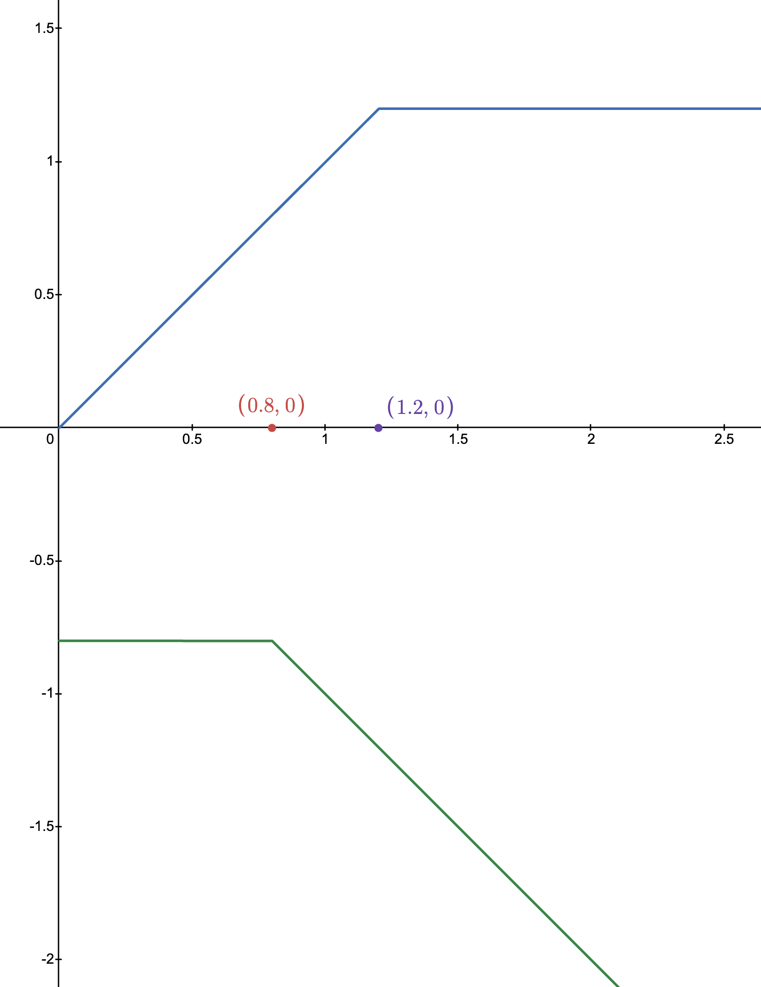
A higher \(r_t(\theta)\) indicates that it is more likely to take \(a_t\) under \(\pi_{\theta}\), hence allowing \(L_t\) to decrease without bound when \(A < 0\) and \(r_t(\theta)\) continues to increase is a sensible decision. On the other hand, for \(A > 0\), when the two policies are about to diverge too much (indicated by \(r_t(\theta) > 1.2\)), we impose a cap on \(L_t\) so that a strong positive, but not unbounded, signal is given.

Let’s now shift gears to LLMs

We’ve come a long way, but so far the discussion has been on general-purpose RL algorithms, rather than about LLMs. Now that we’ve surveyed the necessary concepts up to PPO, we are a good position to talk in the RLHF setting, and specifically how PPO comes into the picture. Specifically, we’ll take a look at PPO, GRPO, and DPO. PPO and GRPO are online RL-style alignment techniques, while DPO is an offline direct preference optimization technique.

Recall that LLMs generate next tokens given a sequence of preceding tokens. RLHF, as we’ve already discussed, is a framework for aligning LLMs with human preferences, commonly post-SFT. Then, using our RL notions,

• LLMs are actors that act based on a policy (in the very beginning of RLHF, they are just \(\pi_{\text{SFT}}\); otherwise we’ll call it \(\pi_\theta\));
• A state \(s_t\) is a prompt \(p\) to the model, plus the generated response up to timestep \(t-1\);
• Taking an action \(a_t\) is equivalent to deciding what the next token would be that continues \(s_t\);
• A reward for the trajectory is the scalar value that can be assigned at the end of the sequence (typically when the model reaches </eos>), measuring how good the response is.

Ingredients of RLHF

To align a model’s responses with human preferences, we should first expose the model with a set of responses that are preferred by humans as well as the dispreferred ones. To do so, we first collect preference datasets. The next question is how to have the model learn which is better and which is worse. The standard approach for doing it is training a reward model (often abbreviated as RM), which outputs a scalar value indicating the quality of the response. Once we have a measurable value, we finally use RL to optimize the policy, using algorithms like PPO that we’ve already seen. Let’s take a closer look at each of these components.

Step 1: Collecting preference datasets

If you have seen interactive elements like this (this one is from Perplexity) while using platforms like ChatGPT or Claude that ask you to judge which of the two responses is better, and have provided your preference, then congratulations, you are a human labeler and have contributed to creating a crowd-sourced preference dataset, which will be used to create a new version of the model that will be released.. perhaps next month!

We will limit our discussion to collecting preference datasets from actual users from the internet, rather than human lebelers that are recruited for this very purpose, for the former option allows for a more resource-efficient mass collection of such dataset. Just to enumerate some ways to create a preference dataset:

1. Provide human labelers with a few different responses to the same prompt and ask them to evaluate them on a scale of 1 (terrible) to 10 (spotless).
2. Same as 1, but on a scale of 1 (terrible) to 5 (spotless).
3. Provide human labelers with a few different responses to the same prompt and ask them to rank them from best to worst.
4. Provide human lebelers with two responses to the same prompt and ask them to decide which is better.

It turns out that requesting human labelers to assign a numeric score to responses can be very tricky. First and foremost, everyone has different standards (just imagine Google or Yelp reviews!) and it is nearly impossible to impose a set standard. Even if such a rubric can be presented to the labeler, it is uncertain whether it is of any notable utility (what if users don’t read it and just click random numers), not to mention that it will result in a significantly degraded UX. Option 3 is an effective workaround, but “best to worst” among more than two responses is still challenging in many scenarios, due to similar reasons. Option 4 is doubtlessly the simplest but is also quite useful in practice (Ziegler et al. (2020)). And of course, we can further extend option 4 by providing the labeler with multiple responses and ask them to select the best one.

Consider a prompt \(x\) and two candidate completions \(y_1, y_2 \sim \pi_{\text{SFT}} (y \mid x)\). We’ll use the notation \(y_p \succ y_d \mid x\) to denote “the labeler has decided that \(y_p\) is a better response compared to \(y_d\) as a response to \(x\)”. A preference dataset is then \(\{ x_i, (y_{i,p}, y_{i,d}) \}_{i=1}^N\) where \(y_{i,p} \succ y_{i,d} \mid x_i\). For instance, the TRL package of Hugging Face recommends that preference datasets be structured as follows:

preference_example = {"prompt": [{"role": "user", "content": "What color is the sky?"}],
                      "chosen": [{"role": "assistant", "content": "It is blue."}],
                      "rejected": [{"role": "assistant", "content": "It is green."}]}

But it should be mentioned that this is not the only valid preference dataset type. For instance, the same TRL package also allows preference datasets to be unpaired, which is compatible with algorithms like KTO, which we will take a look at soon. Don’t forget to check out the full documentation for a comprehensive list of dataset types!

Step 2: Reward Modeling

A reward is a scalar value, but the signal we have in our preference dataset is a binary one, or a pairwise comparison. In order for a signal to be very useful in tuning the LLM’s policy, we need a procedure that maps this binary signal to a scalar reward, and that’s what the reward modeling step is for. Our objective is to train a model that outputs a single scalar given an entire response.

We first assume that there exists a latent reward model \(r^\ast(y, x)\) from which these preferences are generated that outputs the reward for a response \(y\) given the prompt \(x\), and our job is to train a reward model \(r_\phi\) parameterized by \(\phi\) that behaves like \(r^\ast\). Our reward model also takes as input a prompt and a candidate response and outputs the scalar reward. Further, a standard assumption that is adopted to model the preferences is the Bradley-Terry model, which states that

$$ P^\ast(y_p \succ y_d \mid x) = \sigma \bigl( r^\ast(x, y_p) - r^\ast(x, y_d) \bigr), $$

where \(\sigma\) is the sigmoid function. The difference between the two rewards takes into account the fact that we should focus on which one is better, as opposed to their respective absolute rewards. \(P(y_p \succ y_d \mid x)\) is also expressed as the softmax over two items (for instance, here) like the following, which is equivalent to the previous one:

$$ P^\ast(y_p \succ y_d \mid x) = \frac{\exp(r^\ast (x, y_p))}{\exp(r^\ast (x, y_p)) + \exp(r^\ast (x, y_d))}. $$

We thus train the reward model like a binary classification problem: maximum likelihood under a Bradley-Terry preference model, by minimizing the negative log-likelihood of the observed human comparisons. The log-likelihood for a single example is \(\log \mathcal L(\phi) = \log \sigma\bigl(r_\phi (x, y_p) - r_\phi (x, y_d)\bigr) \), and we average over the dataset \(\mathcal D\) to obtain

$$ \mathcal L_R (r_\phi, \mathcal D) = -\mathbb E_{ (x, y_p, y_d) \sim \mathcal D } \bigl[ \log \sigma \bigl( r_\phi (x, y_p) - r_\phi (x, y_d) \bigr) \bigr] $$

The final detail about the reward model is: so what kind of network do we use for \(r_\phi\)? Oftentimes, \(r_\phi\) is just the SFT model (\(\pi_{\text{SFT}}\)), but with the addition of a linear layer on the top whose output dimension is a one-dimensional scalar representing the reward.

Step 3: The RL part

We now have all the necessary ingredients to optimize the policy:

• The reference model \(\pi_{\text{ref}}\), which is the SFT model in our case
• The policy model to optimize \(\pi_\theta\), which we’ll constrain to be similar to \(\pi_{\text{SFT}}\)
• The trained reward model \(r_\phi\), which predicts the reward for the trajectory
• The critic \(V_\psi\), which is updated along with \(\pi_\theta\) to predict the expected return / reward-to-go from that token onward

Step 3.1: Define the RLHF objective

The RLHF objective is as follows:

$$ J_{\text{RLHF}}(\theta) = \mathbb E_{x, y} \Bigl[ r_\phi(x, y) - \beta D_{\text{KL}} \bigl( \pi_\theta(y \mid x) \, \lVert \, \pi_{\text{ref}}(y \mid x) \bigr) \Bigr] $$

where \(x\) is the sampled prompt and \(y\) is the response to the prompt under \(\pi_\theta\). Notice that our objective is not a simple reward maximization; in addition to that, we also want \(\pi_\theta\) to not drift too far from \(\pi_{\text{SFT}}\).

We often approximate \(D_{\text{KL}} \bigl( \pi_\theta(y \mid x) \, \lVert \, \pi_{\text{ref}}(y \mid x) \bigr) \) with \( \log \dfrac{\pi_\theta(y \mid x)}{\pi_{\text{ref}}(y \mid x) } \), for the per-sample log-ratio is a Monte Carlo estimator of the KL integrand whose expectation under \(y \sim \pi_\theta\) equals the KL. This allows us to express \(J_{\text{RLHF}} (\theta)\) as⁹9 Recall that our RL objective has always been to maximize the expected cumulative reward, so this expression is no different than \(\mathbb E_{\tau \sim \pi_\theta} \bigl[ R(\tau) \bigr]\) but we make use of our trained reward function \(r_\phi\) while ensuring the change is not too extreme. In any case, we do not update the weights of \(r_\phi\).

$$ J_{\text{RLHF}} (\theta) = \mathbb E_{x, y} \Bigl[ r_\phi(x, y) - \beta \sum_{t=1}^T \bigl( \log \pi_\theta(a_t \mid s_t) - \log \pi_{\text{ref}} (a_t \mid s_t) \bigr) \Bigr]. $$

One might have noticed that this looks quite different from our PPO clipped surrogate objective, and the reason behind that is because the RLHF objective defines what reward or preference-aligned behavior we want, not the exact SGD loss used in PPO. In other words, \(J_{\text{RLHF}} (\theta)\) is the true conceptual alignment objective, but it is the PPO surrogate that we actually optimize. We’ll get there very soon.

Step 3.2: Go from sequence-level to token-level

Notice that as before, our objective is sequence-level, which is a little divergent from what we actually want in practice. LLMs output token by token, and the response can go off the rails anytime depending on a single “weird” token that is selected, so we need a way to turn the sequence-level signal to a token-level reward.

A common way of doing that is:

• Use KL penalty for non-final tokens, i.e. \(t < T\) (notice that we need to use \(\pi_{\theta_{\text{old}}}\), not \(\pi_\theta\), consistent with the PPO setup): $$ \tilde{r}_t = -\beta \bigl( \log \pi_{\theta_{\text{old}}} (a_t \mid s_t) - \log \pi_{\text{ref}} (a_t \mid s_t) \bigr) $$
• Use the trajectory reward for the final token in addition to the usual KL penalty applied for non-final tokens: $$ \tilde{r}_T = r_\phi(x, y) - \beta \bigl( \log \pi_{\theta_{\text{old}}} (a_T \mid s_T) - \log \pi_{\text{ref}} (a_T \mid s_T) \bigr) $$

This split allows us to define the sum or token-level rewards:

$$ \sum_{t=1}^T \tilde{r}_t = r_\phi(x, y) - \beta \sum_{t=1}^T \bigl( \log \pi_{\theta_{\text{old}}} (a_t \mid s_t) - \log \pi_{\text{ref}} (a_t \mid s_t) \bigr) $$

Step 3.3: Compute rewards-to-go

For PPO, we need to get the advantages \(\hat{A}_t = R_{\geq t} - V_\psi (s_t)\). I might’ve abused the notation here, but \(R_{\geq t}\) denotes the reward-to-go. As we’ve discussed before, at each timestep, we should really focus not on the past returns but the future RLHF reward from token \(t\) onward, hence \(R_{\geq t}\).

$$ R_{\geq t} = \sum_{t' = t}^T \gamma^{t'-t} \tilde{r}_{t'} $$

where the discount factor \(\gamma\) is often set to 1 in RLHF. This formula makes sense; consider for instance the situation with \(T = 5\) and \(t = 3\), in which case we end up with

$$ R_{\geq 3} = \tilde{r}_3 + \gamma^1 \tilde{r}_4 + \gamma^2 \tilde{r}_5 $$

as desired.

Step 3.4: Compute advantage function \(\hat{A}_t\) and GAE

Recall that \(A(s_t, a_t) = Q(s_t, a_t) - V(s)\), whose Monte Carlo estimate is \(\hat{A}_t = G_t - b(s_t)\), where \(b(s_t)\) is the value function, which the critic learns to estimate (recall \( V_\psi (s_t) \approx \mathbb E \left[ G_t \mid s_t \right] \)). The simplest formula would be \(\hat{A}_t = G_t - V_\psi (s_t)\), but in practice we use the generalized advantage estimate (GAE), defined as follows:

$$ \begin{align*} \delta_t &= \tilde{r}_t + \gamma V_\psi(s_{t+1}) - V_\psi(s_t) \\ \hat{A}_t &= \delta_t + (\gamma \lambda) \delta_{t+1} + (\gamma \lambda)^2 \delta_{t+2} + \cdots \end{align*} $$

We’ve already introduced the TD residual \(\delta_t\) briefly here. The generalized advantage estimate combines TD residuals with a rolling sum with an adjustable knob \(\lambda\). If \(\lambda = 0\), \(\hat{A}_t = \delta_t\), equivalent to the single-step TD; if \(\lambda = 1\), we have \(\hat{A}_t = \sum_{l=0}^{T-t} (\gamma)^{l} \delta_{t+l}\), which is the Monte Carlo advantage estimator \(G_t - V(s_t)\) in the finite-horizon case.

We now have the values computed by our advnatage function that tells us whether the sampled token \(a_t\) was better or worse than expected under the RLHF-shaped reward.

Step 3.5: Optimize policies using \(\hat{A}_t\)

The last step is to use the PPO’s clipped surrogate to update \(\pi_\theta\). To copy over the formula we’ve seen before with a simple change from \(\mathbb E\) to \(\hat{\mathbb E}\) (empirical expectation):

$$ \hat{\mathbb E}_t \Bigl[ \min \bigl( r_t(\theta) \hat{A}_t, \textbf{clip}\bigl( r_t(\theta), [1 - \epsilon, 1 + \epsilon] \bigr) \hat{A}_t \bigr) \Bigr]. $$

We’ll include two additional terms to this PPO objective:

1. Entropy bonus: This term behaves as a regularizer that discourages premature collapse or overconfidence (much like having the RL agent explore). To achieve that, we include an entropy bonus that penalizes low entropy.

   $$ L_{\text{entropy}} = \hat{\mathbb E} \left[ H(\pi_\theta(\,\cdot \mid s_t)) \right] $$

   where \( H(\pi_\theta(\, \cdot \mid s_t)) = - \sum_a \pi(a \mid s) \log \pi(a \mid s) \).

2. Critic loss: Recall that we simultaneously update the critic to better predict the value function, so we frame it as a simple MSE loss:

   $$ L_{V} = \hat{\mathbb E} \bigl[ (V_\psi(S_t) - G_t)^2 \bigr]. $$

Combining everything together, we have:

$$ L_{\text{total}} = -L_{\text{RLHF}}^{\text{PPO}} (\theta) + c_V L_V - c_e L_{\text{entropy}}. $$

Notice that we often minimize losses, hence the \(+\) sign in front of the \(L_V\) term, and the \(-\) sign in front of the \(L_{\text{RLHF}}^{\text{PPO}}\) and the \(L_{\text{entropy}}\) term.

GRPO

GRPO, a variant of the PPO algorithm, was introduced in the DeepSeekMath paper. Again, the best “short introduction to GRPO” is from its introduction:

GRPO foregoes the critic model, instead estimating the baseline from group scores, significantly reducing training resources.

With the details already laid out, we can immediately tell what GRPO does: it doesn’t estimate the baselines (required to compute the advantage) using the critic \(V_\psi\) but does it some other way, namely from group scores. The following diagram from the GRPO paper highlights the high-level distinction in an excellent way:

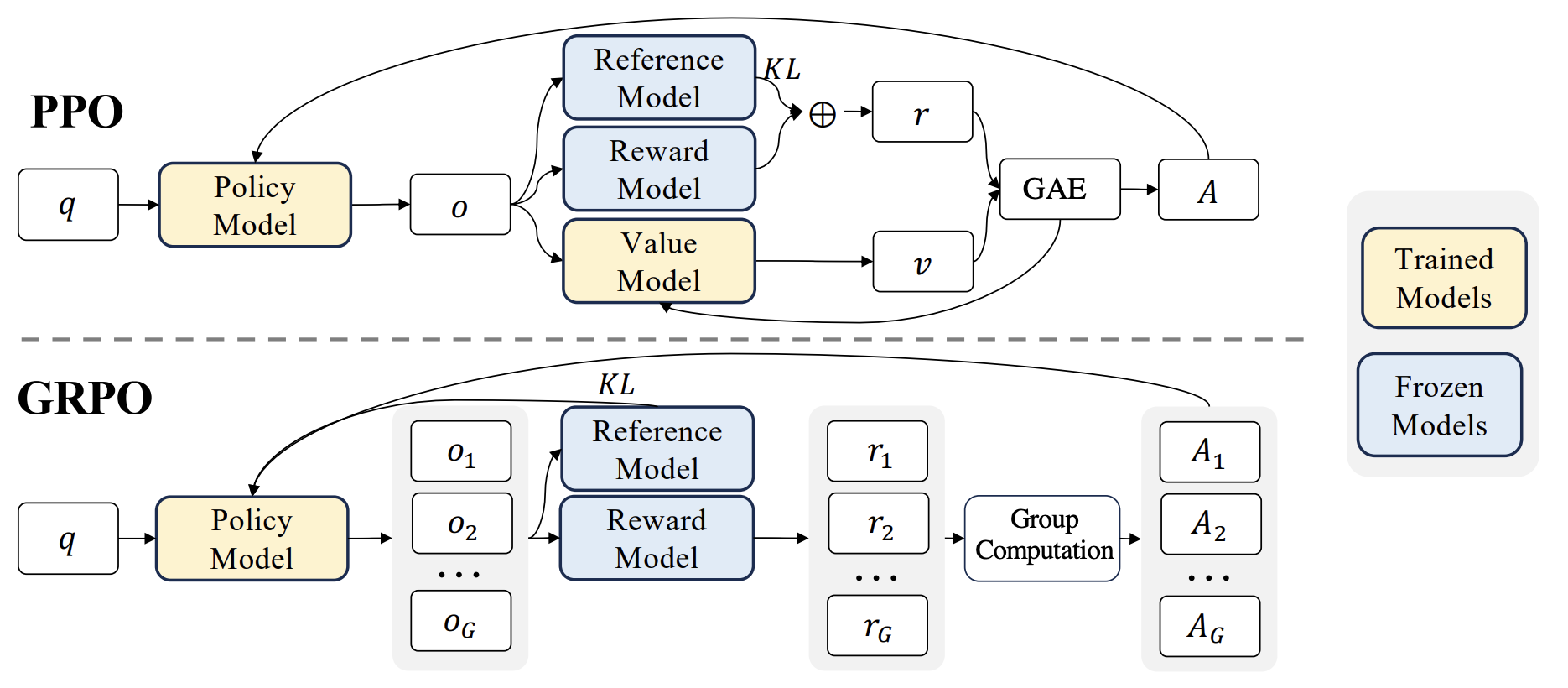
FOR GRPO, instead of learning a critic to estimate a baseline, we sample a group of completions for the same prompt. Based on \(G\) responses to a prompt, \(\{y_1, \cdots, y_G\} \sim \pi_{\theta_{\text{old}}} (\cdot \mid x)\), we compute their rewards (one for each response), and define an advantage-like relative score. Put formally, GRPO replaces critic-based advantage estimation with a group-relative signal.

Let’s make this slightly more explicit. For \(y_1, \cdots, y_G \sim \pi_{\theta_{\text{old}}}(\cdot \mid x)\),

$$ \begin{rcases} r_1 =r_\phi(x, y_1) \quad \\ \qquad \quad \vdots \\ r_G = r_\phi(x, y_G) \end{rcases} \Longrightarrow \tilde{A}_i = \frac{r_i - \text{mean}(r_1, \cdots, r_G)}{\text{stdev}(r_1, \cdots, r_G)}. $$

The GRPO surrogate objective thus differs slightly from that of PPO:

$$ \hat{\mathbb E}_{i,t} \Bigl[ \min \bigl( r_{i,t}(\theta) \tilde{A}_i, \textbf{clip}\bigl( r_{i,t}(\theta), [1 - \epsilon, 1 + \epsilon] \bigr) \tilde{A}_i \bigr) \Bigr] $$

where \(r_{i,t}(\theta)\) denotes the token-level policy ratio for \(y_i\).

DPO

Following suit, let’s take a look at the abstract of the DPO paper (Rafailov et al. (2024)):

RLHF is a complex and often unstable procedure, first fitting a reward model that reflects the human preferences, and then fine-tuning the large unsupervised LM using reinforcement learning to maximize this estimated reward without drifting too far from the original model. In this paper we introduce a new parameterization of the reward model in RLHF that enables extraction of the corresponding optimal policy in closed form, allowing us to solve the standard RLHF problem with only a simple classification loss. The resulting algorithm, which we call Direct Preference Optimization (DPO), is stable, performant, and computationally lightweight, eliminating the need for sampling from the LM during fine-tuning or performing significant hyperparameter tuning.

A core distinction to highlight from this excerpt is the distinction between RLHF and DPO, as well as what the authors of DPO propose to break the complexity of RLHF. RLHF, as we’ve seen, requires training a separate reward model followed by policy optimization algorithms (such as PPO) to adjust the policy. DPO Avoids fitting an explicit standalone reward model and avoids online RL-style policy optimization; it uses a Bradley-Terry preference model (which we’ve already seen above), together with a reward/policy reparameterization that yields the closed-form optimal policy relation. Let’s see how they did it!

Our starting point is \(J_{\text{RLHF}}(\theta)\). To copy it over here again for reference, we want

$$ \begin{align*} \max_{\theta} J_{\text{RLHF}}(\theta) = \max_{\theta} \mathbb E_{x, y} \biggl[ r_\phi(x, y) - \beta D_{\text{KL}} \bigl( \pi_\theta(y \mid x) \, \lVert \, \pi_{\text{ref}} (y \mid x) \bigr) \biggr] \end{align*} $$

Then, as we did above, replacing the KL divergence by its single-sample log-ratio estimator inside the expectation,

$$ \begin{align*} &= \max_\theta \mathbb E_{x, y} \biggl[ r_\phi(x, y) - \beta \log \frac{\pi_\theta(y \mid x)}{\pi_{\text{ref}} (y \mid x)} \biggr] \\ &= \min_\theta \mathbb E_{x, y} \biggl[ -\frac{1}{\beta} r_\phi(x, y) + \log \frac{\pi_\theta(y \mid x)}{\pi_{\text{ref}} (y \mid x)} \biggr]. \end{align*} $$

Let us define a partition function \(Z(x)\) where

$$ Z(x) = \sum_y \pi_{\text{ref}} (y \mid x) \exp \left( \frac{1}{\beta} r_\phi(x, y) \right), $$

then

$$ \begin{align*} &\min_\theta \mathbb E_{x, y} \biggl[ -\frac{1}{\beta} r_\phi(x, y) + \log \frac{\pi_\theta(y \mid x)}{\pi_{\text{ref}} (y \mid x)} \biggr] \\ =& \min_\theta \mathbb E_{x, y} \left[ -\log \exp \left( \beta^{-1} r_\phi(x, y) \right) + \log \frac{\pi_\theta(y \mid x)}{\pi_{\text{ref}} (y \mid x)} \right] \\ =& \min_\theta \mathbb E_{x, y} \left[ \log \frac{\pi_\theta(y \mid x)}{ \pi_{\text{ref}}(y \mid x) \exp \left( \beta^{-1} r_\phi(x, y) \right)} \right] \\ =& \min_\theta \mathbb E_{x, y} \left[ \log \frac{\pi_\theta(y \mid x)}{ \pi_{\text{ref}}(y \mid x) \exp \left( \beta^{-1} r_\phi(x, y) \right)} + \log Z(x) - \log Z(x) \right] \\ =& \min_\theta \mathbb E_{x, y} \left[ \log \frac{\pi_\theta(y \mid x)}{ \frac{1}{Z(x)} \pi_{\text{ref}}(y \mid x) \exp \left( \beta^{-1} r_\phi(x, y) \right)} - \log Z(x) \right] \\ =& \min_\theta \mathbb E_{x} \left[ \mathbb E_{y} \left[ \log \frac{\pi_\theta(y \mid x)}{ \frac{1}{Z(x)} \pi_{\text{ref}}(y \mid x) \exp \left( \beta^{-1} r_\phi(x, y) \right)} \right] - \log Z(x) \right] \\ =& \min_\theta \mathbb E_{x} \left[ D_{\text{KL}} \left( \pi_\theta(y \mid x) \, \middle\| \, \frac{1}{Z(x)} \pi_{\text{ref}}(y \mid x) \exp \left( \beta^{-1} r_\phi(x, y) \right) \right) - \log Z(x) \right] \end{align*} $$

from which we can conclude that the optimal solution \(\pi^\ast (y \mid x)\) is obtained when

$$ \pi^\ast(y \mid x) = \pi_\theta(y \mid x) = \frac{1}{Z(x)} \pi_{\text{ref}}(y \mid x) \exp \left( \beta^{-1} r_\phi(x, y) \right) $$

for all \(x \in \mathcal D\). The only issue with this expression in practice is that \(Z(x)\) is an intractable quantity. But what if we can somehow get rid of \(Z(x)\)?

$$ \begin{align*} Z(x) \pi_\theta(y \mid x) &= \pi_{\text{ref}} (y \mid x) \exp \left( \beta^{-1} r_\phi(x, y) \right) \\ \log Z(x) + \log \pi_\theta(y \mid x) &= \log \pi_{\text{ref}} (y \mid x) + \beta^{-1} r_\phi(x, y) \\ r_\phi(x, y) &= \beta \log Z(x) + \beta \log \pi_\theta (y \mid x) - \beta \log \pi_{\text{ref}} (y \mid x) \\ &= \beta \log \frac{\pi_\theta (y \mid x)}{\pi_{\text{ref}} (y \mid x)} + \beta \log Z(x) \end{align*} $$

And just applying the same logic to derive our latent reward model \(r^\ast(x, y)\) yields

$$ r^\ast(x, y) = \beta \log \frac{\pi^\ast (y \mid x)}{\pi_{\text{ref}} (y \mid x)} + \beta \log Z(x). $$

Recall that according to the Bradley-Terry model,

$$ \begin{align*} P^\ast(y_p \succ y_d \mid x) &= \sigma \bigl( r^\ast(x, y_p) - r^\ast(x, y_d) \bigr) \\ &= \sigma \left( \beta \log \frac{\pi^\ast(y_p \mid x)}{\pi_{\text{ref}}(y \mid x)} \cancel{+ \beta \log Z(x)} - \beta \log \frac{\pi^\ast(y_d \mid x)}{\pi_{\text{ref}}(y \mid x)} \cancel{- \beta \log Z(x)} \right) \\ &= \sigma \left( \beta \log \frac{\pi^\ast(y_p \mid x)}{\pi_{\text{ref}}(y_p \mid x)} - \beta \log \frac{\pi^\ast(y_d \mid x)}{\pi_{\text{ref}}(y_d \mid x)} \right). \end{align*} $$

The derivation above has effectively turned the reward model into the probability of human preference data in terms of the optimal policy, so we can now finally write a clean DPO objective, minimizing the negative log-likelihood loss:

$$ L_{\text{DPO}}(\theta) = -\mathbb E_{(x, y_p, y_d) \sim \mathcal D} \left[ \log \sigma \left( \beta \log \frac{\pi_\theta (y_p \mid x)}{\pi_{\text{ref}}(y_p \mid x)} - \beta \log \frac{\pi_\theta (y_d \mid x)}{\pi_{\text{ref}}(y_d \mid x)} \right) \right]. $$